A Brief Overview of Parallelism Strategies in Deep Learning

Royal York Crescent, Bristol.

It has been nearly half a year since I started my first real job as a fully-fledged graduate. This has taken the form of being an AI Engineer at Graphcore, a Bristol-based AI accelerator startup. In quite a short amount of time, I have learned a great great deal and I am grateful for the opportunity and the patience of my colleagues – the latter of which is particularly needed when tutoring the average, fresh compsci graduate.

Chief among what I have learned is a wide array of parallelism strategies. If you are at least somewhat familiar with Graphcore’s IPU accelerators, you will know why. But for the uninitiated, the amount of on-chip memory that can be directly accessed without hassle on an IPU, is considerably smaller than the GPUs of today. Luckily, it has a substantial amount of secondary DRAM memory - also on IPU - so offloading is faster than it would be to CPU. Nevertheless, though the IPU has a number of advantages versus a GPU, the reduced size does mean that resorting to parallelism is more common.

Though that doesn’t sound great, if you stop to consider the fast growing model sizes in the deep learning community, you will maybe notice that this isn’t a huge deal if you are interested in large models. Why is that? Because now mass parallelism is also required on GPUs. Huge scales are the great equaliser it seems, and a single accelerator of any type can do nought next to the likes of GPT-3, PaLM, Parti, and friends.

This is exactly the position I found myself in when I landed in Graphcore, aligning myself quickly on the large model side of things. Conceptually, parallelism in deep learning is not tricky, but regarding implementations I still have a ways to go. For now though, I will share what I have learned on this topic.

Luckily, the concepts are agnostic to the type of compute device used – you could even treat everything as a desktop CPU, or a graphing calculator – so this will not be IPU specific nor even framework specific, only high-level concepts. This means I will not include code examples, but I will link to tutorials and frameworks that implement the concepts I discuss at the end of each section.

Working with a Single Device

It’s helpful to begin with the single device case. One host (a regular PC with a CPU and memory), one accelerator we want to run our model on, suppose a GPU, which has its own processing and memory components. During execution, we load parameters and data onto the device, and create intermediate data on-device such as activations and gradients. If you are a deep learning practioner you should be familiar with this scenario.

You will also be familiar with this other scenario:

> x = torch.empty(int(1e12), device=device)
OutOfMemoryError: CUDA out of memory. Tried to allocate 3725.29 GiB (GPU 0;
23.69 GiB total capacity; 3.73 GiB already allocated; 18.56 GiB free; 3.75 GiB
reserved in total by PyTorch) If reserved memory is >> allocated memory try
setting max_split_size_mb to avoid fragmentation.  See documentation for Memory
Management and PYTORCH_CUDA_ALLOC_CONF

For which you probably have a few solutions you immediately reach for, such as a credit card.

On-device memory is typically used for the following things:

• Storing model parameters.
• Storing activations.
• Storing gradients.
• Storing optimiser states.
• Storing code.

Having to store gradients and optimiser states on-device is one reason why training models uses more memory than just running inference. This is particularly true for more advanced (read: memory-hungry) optimisers like Adam.

And potential solutions include the following:

• Switch to a lower floating point precision :right_arrow: less bits used per tensor.
• Decrease micro-batch size and compensate with gradient accumulation :right_arrow: reduces size of activations and gradients.
• Turn on “no gradient” or “inference mode” :right_arrow: only store current activations, no gradients stored. Clearly inference only.
• Sacrifice extra compute for memory savings (ex: recomputation of activations, attention serialisation)
• CPU offload :right_arrow: only load tensors onto device when needed, otherwise store in host memory.

..among others!

These solutions help a lot in most workflows and can allow for training much larger models on a single device than you would expect (see this Microsoft blog). However, for one reason or another, this is sometimes just not practical or has other downsides such as training instability. In such cases, resorting to parallelism may be necessary.

Data Parallelism

Arguably one of the simplest forms of parallelism, data parallelism simply takes all the devices you have, copies model and optimiser parameters and code onto all of them, then sends different micro-batches to each device. Gradients are then synchronised between devices, followed by an optimiser step, resulting in parameter updates. In essence, we use more devices to chew through the dataset faster, thus obtaining a speedup. It also enables larger (global) batch sizes without performing too many gradient accumulation iterations.

Note, that the model and optimiser parameters are replicated on all devices (all replicas). Hence, in order for this parallelism to work, we need to be able to fit the entire model with a micro-batch size of at least one on a single replica.

Data parallelism won’t directly help fit larger models, but can help increase the batch size that you likely had to reduce to squeeze the model in originally. My first encounter with this was during my master’s dissertation, training a VQ-GAN model, where I could only train on a single device with a micro-batch size of one, but could obtain a global batch size of 16 with 4 devices and 4 gradient accumulation steps.

Data parallelism is also relatively communication light, as we only need to all-reduce the gradients whenever we update the optimiser, which could be infrequent depending on the number of gradient accumulation steps. This also reduces the need for high-speed interconnect between replicas, as communication is infrequent.

To use data parallelism in your code see this post for PyTorch fans and this post for Jax. I also like this post by Kevin Kai-chuang for PyTorch. However, by far the easiest way to add data parallelism to your code in PyTorch is to use Huggingface Accelerate which near-perfectly abstracts away data parallelism, and integrates with powerful libraries like Deepspeed, right out of the box.

Pipeline Parallelism

Pipeline Parallelism is used when the entire model is too large to fit on a single device. The model is split into stages and each stage executed on a different device, passing activations between neighbouring stages when a boundary is reached during execution.

For inference, this is extremely good for improving total throughput of the system as multiple micro-batches can be processed in parallel, with communication only happening at stage boundaries. Sometimes, even if the model fits on one device, pipelining can be used to improve throughput like this (at the cost of latency).

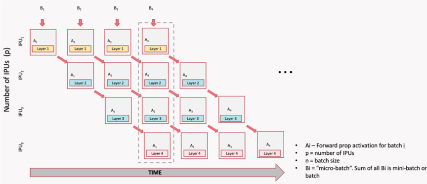
Shamelessly taken from a tutorial from my job. Same goes for all images in this section on pipelining.

There is a noticeable gap at the start of the above inference pipeline. This is known as the ramp-up phase where device utilisation cannot be at 100%. Clearly stage 3 cannot begin executing micro-batch 1 until stage 1 and 2 are both done with micro-batch 1. However, in this scheme, once the final stage $N$ has received the first micro-batch, we reach the main phase and reach maximum utilisation. Once the first stage processes the final micro-batch, we reach the ramp-down stage, as their is simply no more data left to execute on.

For best utilisation, the time to execute each stage should be as balanced as possible. This is because if one stage finishes early, it may have to wait for the subsequent stage to be ready before passing on its activations and executing its next micro-batch. This is easy in relatively homogeneous models like transformers, where most layers are typically the same size, but difficult in other models such as Resnets or UNets.

How does this extend to training?

It makes sense for each stage $t$ to also handle its own backwards pass $t$, so we don’t need to copy activations or parameters to multiple devices. However, one problem is that we cannot handle the backwards for a stage $t$, without having the results for backwards $t+1, \dots, N$ and the forwards for $t-1, \dots, 1$.

Let’s begin with the simplest scheme that meets these conditions:

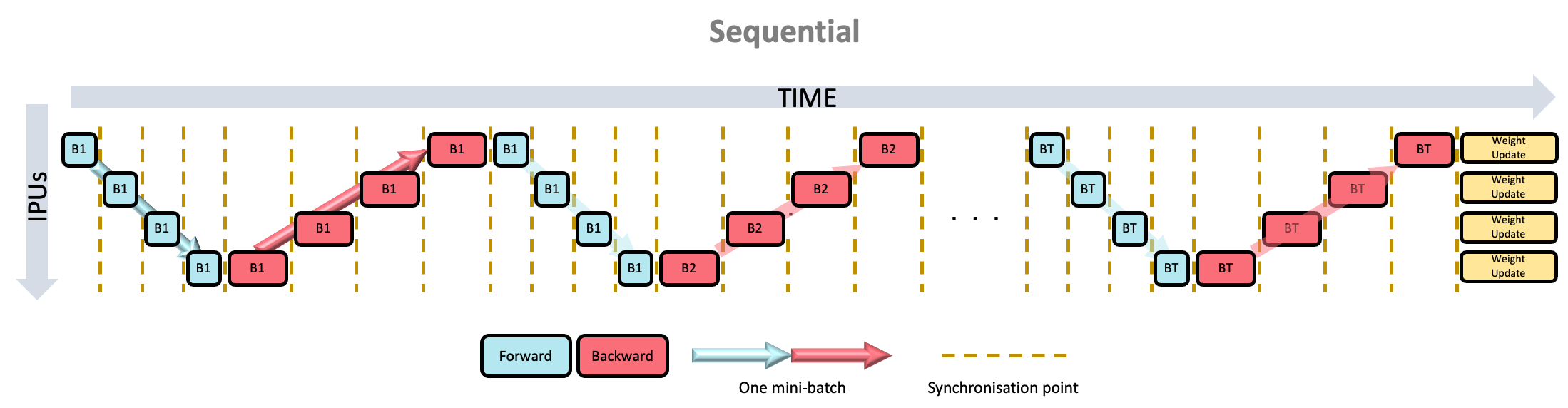
Yes, the second set for forward should probably say “B2”.

In this scheme, only one micro-batch is in play at a time, leaving all stages but one idle. After finishing the final stage, we turn around and begin the backwards pass, again leaving all but one stage idle. Once a full batch is computed (in other words, after the ramp-down), a weight update is performed. This means the utilisation is always going to be (at most) $1/N$ of full utilisation. Clearly extremely inefficient!

However, good for debugging purpose!

We can do better with a grouped pipeline:

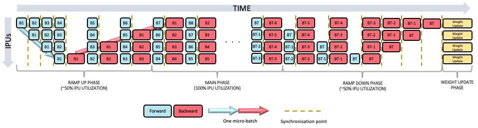
The ramp-up phase almost consists of two “sub-ramp-ups”: the first being the same as the inference ramp-up, followed by a ramp-up of the backwards passes which alternate with main-phase forward passes. Once the main-stage is reached, we alternate between forward and backwards passes on all stages.

We can alternate as once a stage $t$ processes the backwards of micro-batch $b$, it can discard activations and accumulate gradients. It is then ready to process the next forward pass for micro-batch $b+1$. Like before, a weight update occurs after a ramp-down phase.

Another approach is to interleave the forwards and backwards passes:

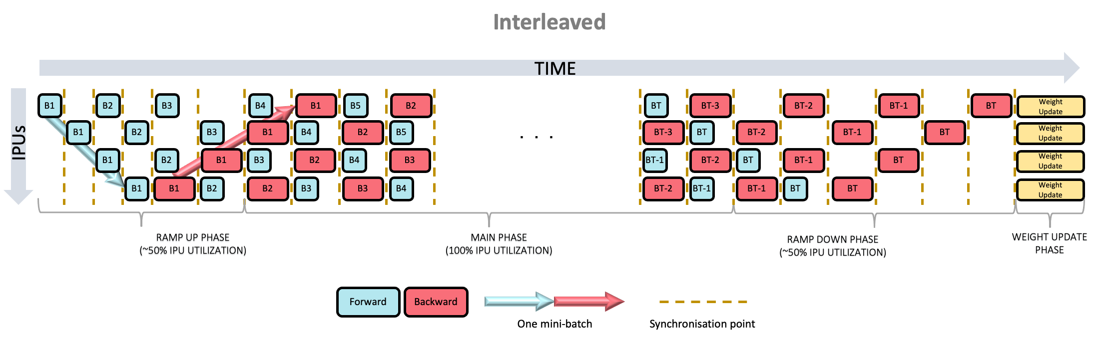
At any given point, half the stages are executing a forward pass, and half a backwards pass. Because of this, the ramp-up and ramp-down phases are much shorter, resulting in a quicker time to maximum utilisation.

The last two schemes have different advantages and disadvantages:

• At any given time, the grouped scheme executes twice as much mini-batches as the interleaved scheme, meaning more memory is required to store activations
• Grouped schemes executes all forward and backwards together, meaning communication is less frequent. Interleaved executes separately, resulting in more communication and also some idle time when forward passes wait for backward passes – which typically take longer than forward passes. Hence, grouped schemes are typically faster than interleaved.
• Interleaved ramp-up and ramp-down time is about twice as fast as grouped, meaning it is quicker to reach full utilisation.

Pipeline parallelism uses much more communication than data parallel, however less than tensor parallelism, which I will discuss in the next section. Communication is limited to boundaries between stages, meaning regardless of the number of stages, each one will send one set of activations, and receive one set. The communication can be done in parallel between all replicas.

PyTorch has native support for pipelining here which uses the GPipe algorithm. This was used to train larger transformer models in this tutorial. Deepspeed provides more advanced pipeline parallelism, which is explained in this tutorial.

Jax, meanwhile, has no native support for pipeline parallelism, but frameworks around Jax such as Alpa do support it, demonstrated in this tutorial. Lack of native support in Jax likely comes from its emphasis on TPUs, which have high bandwidth interconnect between all replicas in a TPU pod (versus GPUs which have fast interconnect only within a host). This means it is preferable to simply use data and tensor parallelism (more on the latter later) so to avoid pipeline bubbles.

Tensor Parallelism

What about if a single layer is too big to fit on a single replica? Say for example, a particularly large MLP expansion, expensive self-attention layer, or a large embedding layer. In such cases, the parameters of a layer can be split across multiple devices. Partial results are then computed on each device before materialising the final result by communicating between the replicas.

Take, for example, the MLP block in a standard transformer model that projects a vector $x$ to and from a space of dimension $d$ and $4d$:

$$h = W_2 \cdot f(W_1 \cdot x + b_1) + b_2 $$ where $f$ is a nonlinear activation function, $W_{*}$ are the weight matrices, and $b_{*}$ are the bias vectors.

To turn this into a tensor parallel layer, do the following:

• Split $W_1$ row-wise into $n$ pieces, sending one to each of $n$ replicas.
• Split $b_1$ into $n$ pieces, as above.
• Split $W_2$ column-wise into $n$ pieces, sending one to each of $n$ replicas.

Then, given an input $x$, do on each replica $i$:

• Compute $f(W_1^{(i)} \cdot x + b_1^{(i)})$, resulting in a vector $z_i$ of size $4d/n$.
• Compute $W_2^{(i)} \cdot z_i$, resulting in $\hat{h_i}$ of size $d$

This, naturally, does not give the same result. The next part resolves this:

• Communicate between replicas to compute $\sum^n_{i=1} \hat{h_i} $
• On all replicas add $b_2$ (which is identical on all replicas), to get the final result $h$ on all replicas.

The first operation sums the partial results across all replicas, which means all replicas have the same value at this point. Then, all replicas identically compute $b_2$, which still results in the same (and correct) result, despite no communication happening after this addition.

A nice exercise is to write out mathematically the operations happening here, and see that we do indeed arrive at the same result. However, I will save myself you the pain here.

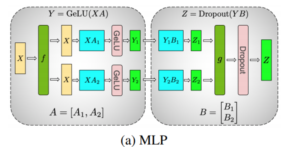
A diagram of a tensor parallel MLP from the Megatron paper.

Another example is an embedding layer in a transformer. We can split the embedding matrix along the vocabulary dimension, resulting in a shards of shape $V/n \times d$. All replicas receive the same input tokens and compute the embedding. However, if any given token falls outside a given replica’s valid range, a zero tensor is instead returned. Then, an all-reduce will rematerialise the final result, as only one replica (for any given element in the input sequence) will have a non-zero tensor.

Other examples include splitting attention heads, convolution channels or even the spatial dimensions themselves, between the replicas.

Regardless of the context tensor parallelism is applied, it should be noted that communication between replicas in the same tensor parallel group occur much more frequently than in data parallel groups or between pipeline stages. This means that time spent communicating compared to actually computing a result increases. Because of this, replicas in the same tensor parallel group should be placed on higher bandwidth interconnect, if possible.

Depending on the model size tensor parallelism can be totally unavoidable, but should be avoided if possible! Of course, exceptions are also possible. One case is where (suppose) you could not use pipeline parallelism, so in order to fit the model onto the available devices, you use tensor parallelism throughout the model, despite no single layer causing an out of memory. This is somewhat orthogonal to pipeline parallelism: splitting through the model rather than across.

Support for tensor parallelism in PyTorch is experimental see this RFC but is supported in Deepspeed as “tensor-slicing model-parallelism”. Tensor parallelism can be achieved in Jax using jax.pjit.

All together now..

A keen eyed reader may have noticed that these parallelism strategies should not be incompatible with one another – perhaps they may even use the term orthogonal. Indeed, when we target very large model sizes, or have a lot of compute to throw around, we start arranging replicas into hierarchies and groups.

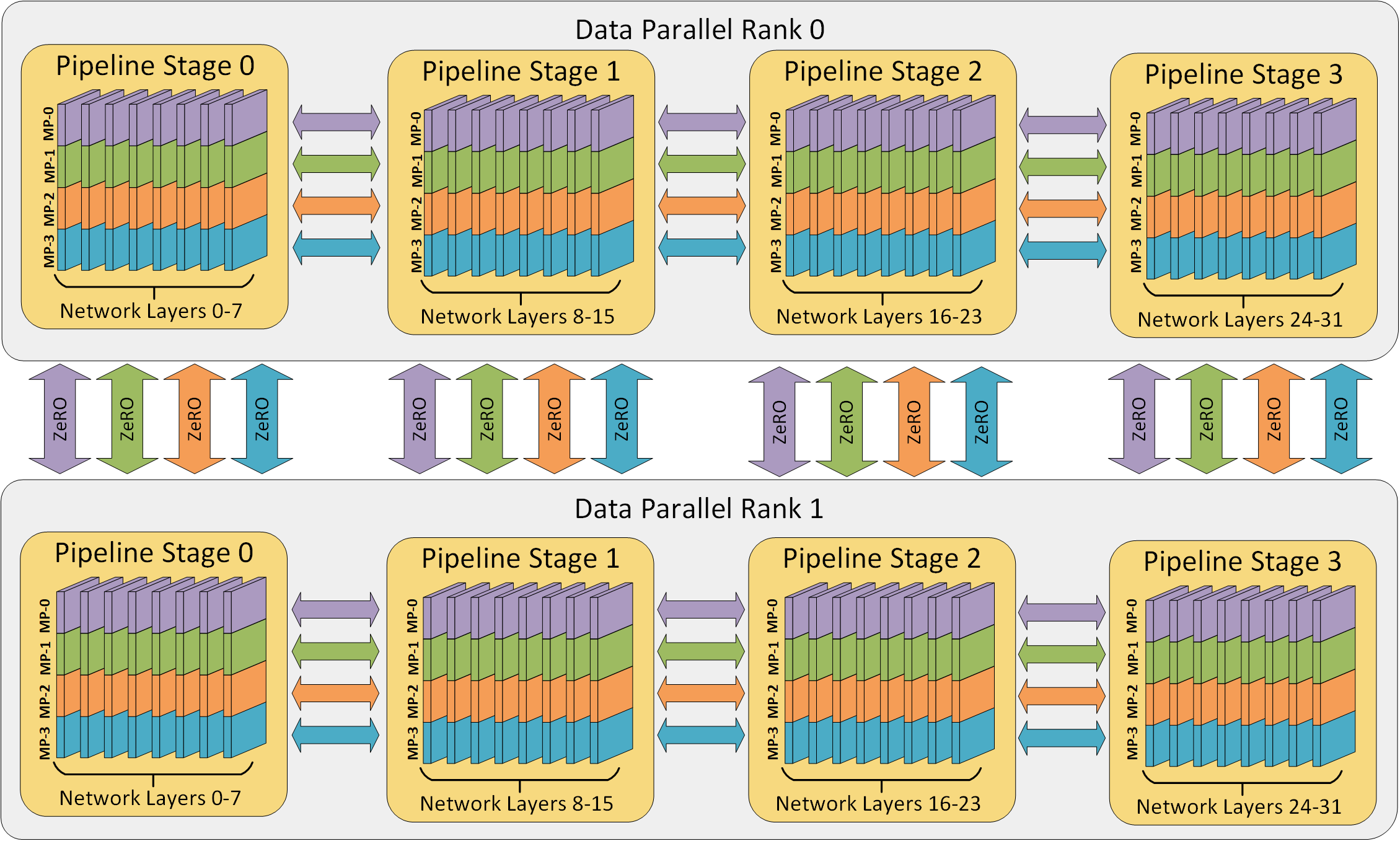
Take for example, a system with a data parallel factor of $n_d$. Each data parallel instance will contain an exact copy of the model – simply sending different batches to each data parallel instance. If we employ pipeline parallelism with $n_p$ pipeline stages, and each data parallel instance contains an exact copy, then each data parallel instance must also contain $n_p$ pipeline stages, giving $n_p \cdot n_d$ replicas total.

Adding tensor parallelism to the mix, splitting layers among $n_t$ replicas, each pipeline stage will use $n_t$ replicas. Naturally, this gives a total number of replicas of $n = n_p \cdot n_d \cdot n_t$. This gives a hierarchy of data parallel at the very top, down to tensor parallelism at the bottom. This also translates near perfectly to a typical compute cluster.

Recall that data parallel communications (the gradient all reduce) occur much less frequently than tensor parallelism communication (potentially multiple times per layer). Furthermore, larger clusters typically consist of multiple nodes, where communication between devices on a single node is much faster than communication between nodes. It therefore makes sense then to group tensor parallel replicas that need to communicate together on a single node, and place ones that do not across nodes. In other words, prioritise placing tensor parallel groups on high-bandwidth interconnect over data parallel groups.

For example, using IPUs, certain IPUs have more links between them and so give a higher speed interconnect. Moreover, certain IPUs exist together on the same motherboard, whereas others only share the same host server, or perhaps even use different host servers entirely. For GPUs, perhaps certain GPUs are connected together using NVLink and others over ethernet between different servers - perhaps even over the internet in a swarm-like style.

Though these parallelism methods are orthogonal to one another, it is still a challenging task to combine them. Moreover, though a certain scheme may make the model fit, it may be terribly inefficient. The problem of taking a model and cluster configuration as input and producing a good grouping of replicas to maximise performance is an art in and of itself. It remains still an active area of research. One such method is Alpa by Google research which has a framework built around Jax here.

Conclusion

Unless something tremendously dramatic happens in deep learning research, very large models are here to stay. Therefore, at least being aware of these techniques will become a fact of life for most AI engineers. Even if the interfaces become very clean in the future (so engineers can just fire-and-forget) there will be still a benefit in knowing how things word under the hood, just like the benefits gained from studying anything we take for granted now.

I am still a beginner in this topic and had never deeply explored before starting my job. Luckily for me I found it very interesting, albeit a little annoying to work with versus working with a single device. There is also a bit of a cognitive shift required to move from a serial execution world, where most people start from, to a massively parallel world, where we are going. Same goes for simply handling such large models: from longer load times to slower development loops to simply comprehending that “if we split the parameters of Bloom among every human being, each one would get 22 parameters”. However, the difficulty is worth it to better understand how large behemoths like GPT-3 are orchestrated.

In the future and as I gain more experience, I would like to dive into further detail about specific methods mentioned here and those yet-to-come. However for now, and given my current experience level, I simply hope this post can help you gain a high-level understanding of the methods currently available to us in deep learning system parallelism.