Easy JAX training loops with Flax and Optax

In my previous blog post, I discussed JAX – a framework for high performance numerical computing and machine learning — in an atypical manner. I didn’t create a single training loop, and only showed a couple patterns that looked vaguely machine learning-like. If you haven’t read that blog post yet, you can read it here.

This approach was deliberate as I felt that JAX — although designed for machine learning research — is more general-purpose than that. The steps to use it are to define what you want to happen, wrap it in within jax.jit, let JAX trace out your function into an intermediate graph representation, which is then passed to XLA where it will be compiled and optimised. The result is a single, heavily-optimised, binary blob, ready and waiting to receive your data. This approach is a natural fit for many machine learning applications, as well as other scientific computing tasks. Therefore, targeting machine learning only didn’t make sense. It is also ground that has already been extensively covered — I wanted to do a different take on introductory JAX.

In the previous post, I mentioned that it is possible to develop a full machine learning training loop — models, optimisers and all — in pure JAX. This is self-evident as JAX is general-purpose. It is a good exercise, but not a strategy I like to employ. In this blog post I want to introduce two higher level libraries built on top of JAX, that do a lot of the heavy lifting for us when writing machine learning applications. These libraries are Flax and Optax.

To summarise the libraries:

• JAX — provides a high-level neural network API that lets the developer reason about the model in terms of components, like in PyTorch, rather than with JAX functions that take parameters as inputs.
• Optax — a library containing a vast array of model training utilities, such as optimisers, loss functions, learning rate schedulers, and more! Very batteries-included.

At the end of this post, we will have implemented and trained a very simple class-conditioned image generation model called a variational autoencoder (VAE) to generate MNIST digits.

Neural Network API with Flax

The high level structure of a training loop in pure JAX, looks something like this:

dataset = ...   # initialise training dataset that we can iterate over
params = ...    # initialise trainable parameters of our model
epochs = ...

def model_forward(params, batch):
    ...         # perform a forward pass of our model on `batch` using `params`
    return outputs

def loss_fn(params, batch):
    model_output = model_forward(params, batch)
    loss = ...  # compute a loss based on `batch` and `model_output`
    return loss

@jax.jit
def train_step(params, batch):
    loss, grads = jax.value_and_grad(loss_fn)(params, batch)
    grads = ...  # transform `grads` (clipping, multiply by learning rate, etc.)
    params = ... # update `params` using `grads` (such as via SGD)
    return params, loss

for _ in range(epochs):
    for batch in dataset:
        params, loss = train_step(params, batch)
        ...         # report metrics like loss, accuracy, and the like.

We define our model in a functional manner: a function that takes the model parameters and a batch as input, and returns the output of the model. Similarly, we define the loss function that also takes the parameters and a batch as input, but returns the loss instead.

Our final function is the train step itself which we wrap in jax.jit – giving XLA maximum context to compile and optimise the training step. This first computes the gradient of the loss function using the function transform jax.value_and_grad, manipulates the returned gradients (perhaps scaling by a learning rate), and updates the parameters. We return the new parameters, and use them on the next call to train_step. This is called in a loop, fetching new batches from the dataset before each training step.

Most machine learning programs follow a pattern such as the one above. But in frameworks like PyTorch, we package together the model forward pass and the management of model parameters into a stateful object representing our model – simplifying the training loop. It would be nice if we could imitate this behaviour in stateless JAX to allow the developer to reason about models in a class-based way. This is what Flax’s neural network API – flax.linen – aims to achieve.

Whether or not writing models in a purely stateless, functional way is better than a stateful, class-based way, is not the topic of this blog post. Both have merits. Regardless, during execution the final result is the same whether we use Flax or not. We get a stateless, heavily-optimised, binary blob that we throw data at. It’s all JAX after all.

There are two main ways to define a module in Flax: one is PyTorch-like and the other is a compact representation:

import flax.linen as nn
from typing import Callable
class Model(nn.Module):
    dim: int
    activation_fn: Callable = nn.relu

    def setup(self):
        self.layer = nn.Dense(self.dim)

    def __call__(self, x):
        x = self.layer(x)
        return self.activation_fn(x)

class ModelCompact(nn.Module):
    dim: int
    activation_fn: Callable = nn.relu

    @nn.compact
    def __call__(self, x):
        x = nn.Dense(self.dim)(x)
        return self.activation_fn(x)     

If we have complex initialisation logic, the former may be more appropriate. Instead, if the module is relatively simple, we can make use of the nn.compact representation to automatically define the module by the forward pass alone.

Like other frameworks, we can nest modules within each other to implement complex model behaviour. Like we’ve already seen, flax.linen provides some pre-baked modules like nn.Dense (same as PyTorch’s nn.Linear). I won’t enumerate them all, but the usual candidates are all there like convolutions, embeddings, and more.

Something to bear in mind if you are porting models from PyTorch to Flax is that the default weight initialisation may be different. For example, in PyTorch the default bias initialisation is the LeCun normal, but in Flax it is initialised to zero.

However, currently we cannot call this model, even if we were to initialise the class itself. There simply aren’t any parameters to use. Furthermore, the module is never a container for parameters. An instance of a Flax module is simply a hollow shell, that loosely associates operations with parameters and inputs that are passed as input later.

To see what I mean, let’s initialise some parameters for our model:

key = jax.random.PRNGKey(0xffff)
key, model_key = jax.random.split(key)

model = Model(dim=4)
params = model.init(model_key, jnp.zeros((1, 8)))
params
===
Out: 
FrozenDict({
    params: {
        layer: {
            kernel: Array([[-0.05412389, -0.28172645, -0.07438638,  0.5238516 ],
                   [-0.13562573, -0.17592733,  0.45305118, -0.0650041 ],
                   [ 0.25177842,  0.13981569, -0.41496065, -0.15681015],
                   [ 0.13783392, -0.6254694 , -0.09966562, -0.04283331],
                   [ 0.48194656,  0.07596914,  0.0429794 , -0.2127948 ],
                   [-0.6694777 ,  0.15849823, -0.4057232 ,  0.26767966],
                   [ 0.22948688,  0.00706845,  0.0145666 , -0.1280596 ],
                   [ 0.62309605,  0.12575962, -0.05112049, -0.316764  ]],      dtype=float32),
            bias: Array([0., 0., 0., 0.], dtype=float32),
        },
    },
})

In the above cell, we first initialised our model class, which returns an instance of Model which we assign to the variable model. Like I said, it does not contain any parameters, it is just a hollow shell that we pass parameters and inputs to. We can see this by printing the model variable itself:

model
===
Out: Model(
    # attributes
    dim = 4
    activation_fn = relu
)

We can also call the module itself, which will fail even though we have defined the __call__ method:

model(jnp.zeros((1, 8)))
===
Out:
/usr/local/lib/python3.10/dist-packages/flax/linen/module.py in __getattr__(self, name)
    935         msg += (f' If "{name}" is defined in \'.setup()\', remember these fields '
    936           'are only accessible from inside \'init\' or \'apply\'.')
--> 937       raise AttributeError(msg)
    938 
    939   def __dir__(self) -> List[str]:

AttributeError: "Model" object has no attribute "layer". If "layer" is defined in '.setup()', remember these fields are only accessible from inside 'init' or 'apply'.

To initialise the parameters, we passed a PRNG key and some dummy inputs to the model’s init function of the same shape and dtype as the inputs we will use later. In this simple case, we just pass x as in the original module’s __call__ definition, but could be multiple arrays, PyTrees, or PRNG keys. We need the input shapes and dtypes in order to determine the shape and dtype of the model parameters.

From the model.init call, we get a nested FrozenDict holding our model’s parameters. If you have seen PyTorch state dictionaries, the format of the parameters is similar: nested dictionaries with meaningful named keys, with parameter arrays as values. If you’ve read my previous blog post or read about JAX before, you will know that this structure is a PyTree. Not only does Flax help developers loosely associate parameters and operations, it also helps initialise model parameters based on the model definition.

With the parameters, we can call the model using model.apply – providing the parameters and inputs:

key, x_key = jax.random.split(key)
x = jax.random.normal(x_key, (1, 8))
y = model.apply(params, x)
y
===
Out: Array([[0.9296505 , 0.25998798, 0.01101626, 0.        ]], dtype=float32)

There is nothing special about the PyTree returned by model.init – it is just a regular PyTree storing the model’s parameters. params can be swapped with any other PyTree that contains the parameters model expects:

zero_params = jax.tree_map(jnp.zeros_like, params) # generates a PyTree with same structure as `params` will all values set to 0.
print(zero_params)
model.apply(zero_params, x)
===
Out:
FrozenDict({
    params: {
        layer: {
            bias: Array([0., 0., 0., 0.], dtype=float32),
            kernel: Array([[0., 0., 0., 0.],
                   [0., 0., 0., 0.],
                   [0., 0., 0., 0.],
                   [0., 0., 0., 0.],
                   [0., 0., 0., 0.],
                   [0., 0., 0., 0.],
                   [0., 0., 0., 0.],
                   [0., 0., 0., 0.]], dtype=float32),
        },
    },
})

Array([[0., 0., 0., 0.]], dtype=float32)

Forcing model calls to require explicitly passing parameters keeps it stateless and returning parameters like any other PyTree, makes Flax interoperable with JAX functions – as well as other libraries built on JAX. Essentially, by using Flax we aren’t forced to use any other specific frameworks and have access to all regular JAX features.

If you are used to frameworks like PyTorch, calling models like this feels unnatural at first. However, I personally quite like it this way – it feels rather elegant to pass different parameters to the model to get different behaviour rather than “load” the weights. A bit subjective and fuzzy, I know, but I like it.

To summarise the difference, if we aim to implement $f_\theta(x)$, a PyTorch module is basically $f_\theta$ (which we can call on $x$). A Flax module is simply $f$, which needs to be provided parameters $\theta$ before it can be called on $x$ – or alternatively, we call $f$ on $(\theta, x)$.

All in all, the point of Flax is to provide a familiar stateful API for development whilst preserving JAX statelessness during runtime. We can build our neural network modules in terms of classes and objects, but the final result is a stateless function model.apply that takes in our inputs and a PyTree of parameters.

This is identical behaviour to what we began with (recall our model_forward function at the start of this section), just now tied up nicely together. Therefore, our function containing model.apply that takes as input our PyTree, can be safely jit-compiled. The result is the same, a heavily-optimised binary blob we bombard with data. Nothing changes during runtime, it just makes development easier for those who prefer reasoning about neural networks in a class-based way whilst remaining interoperable with, and keeping the performance of JAX.

There’s a lot more to Flax than this, especially outside the flax.linen neural network API. For now though, we will move on to developing a full training loop using Flax and Optax. We will swing back around to some extra Flax points later, but I feel some concepts are hard to explain without first showing a training loop.

A full training loop with Optax and Flax

We’ve shown how to reduce the complexity of writing model code and parameter initialisation. We can push this further by relying on Optax to handle the gradient manipulation and parameter updates in train_step. For simple optimisers, these steps can be quite simple. However, for more complex optimisers or gradient transformation behaviour, it can get quite complex to implement in JAX alone. Optax packages this complex behaviour into a simple API.

import optax
optimiser = optax.sgd(learning_rate=1e-3)
optimiser
===
Out: GradientTransformationExtraArgs(init=<function chain.<locals>.init_fn at 0x7fa7185503a0>, update=<function chain.<locals>.update_fn at 0x7fa718550550>)

Not pretty, but we can see that the optimiser is just a gradient transformation – in fact all optimisers in Optax are implemented as gradient transformations. A gradient transformation is defined to be a pair of functions init and update, which are both pure functions. Like a Flax model, Optax optimisers have no state kept internally, and must be initialised before it can be used, and any state must be passed by the developer to update:

optimiser_state = optimiser.init(params)
optimiser_state
===
Out: (EmptyState(), EmptyState())

Of course, as SGD is a stateless optimiser, the initialisation call simply returns an empty state. It must return this to maintain the API of a gradient transformation. Let’s try with a more complex optimiser like Adam:

optimiser = optax.adam(learning_rate=1e-3)
optimiser_state = optimiser.init(params)
optimiser_state
===
Out: (ScaleByAdamState(count=Array(0, dtype=int32), mu=FrozenDict({
     params: {
         layer: {
             bias: Array([0., 0., 0., 0.], dtype=float32),
             kernel: Array([[0., 0., 0., 0.],
                    [0., 0., 0., 0.],
                    [0., 0., 0., 0.],
                    [0., 0., 0., 0.],
                    [0., 0., 0., 0.],
                    [0., 0., 0., 0.],
                    [0., 0., 0., 0.],
                    [0., 0., 0., 0.]], dtype=float32),
         },
     },
 }), nu=FrozenDict({
     params: {
         layer: {
             bias: Array([0., 0., 0., 0.], dtype=float32),
             kernel: Array([[0., 0., 0., 0.],
                    [0., 0., 0., 0.],
                    [0., 0., 0., 0.],
                    [0., 0., 0., 0.],
                    [0., 0., 0., 0.],
                    [0., 0., 0., 0.],
                    [0., 0., 0., 0.],
                    [0., 0., 0., 0.]], dtype=float32),
         },
     },
 })),
 EmptyState())

Here, we can see the first and second order statistics of the Adam optimiser, as well as a count storing number of optimiser updates. Like with SGD, this state needs to be passed to update when called.

Like Flax parameters, the optimiser state is just a PyTree. Any PyTree with a compatible structure could also be used. Again, this also allows interoperability with JAX and jax.jit, as well as other libraries built on top of JAX.

Concretely, Optax gradient transformations are simply a named tuple containing pure functions init and update. init is a pure function which takes in an example instance of gradients to be transformed and returns the optimiser initial state. In the case of optax.sgd this returns an empty state regardless of the example provided. For optax.adam, we get a more complex state containing the first and second order statistics of the same PyTree structure as the provided example.

update takes in a PyTree of updates with the same structure as the example instance provided to init. In addition, it takes in the optimiser state returned by init and optionally the parameters of the model itself, which may be needed for some optimisers. This function will return the transformed gradients (which could be another set of gradients, or the actual parameter updates) and the new optimiser state.

This is explained quite nicely in the documentation here

Providing some dummy data, we get the following:

import optax
params = jnp.array([0.0, 1.0, 2.0]) # some dummy parameters
optimiser = optax.adam(learning_rate=0.01)
opt_state = optimiser.init(params)

grads = jnp.array([4.0, 0.6, -3])# some dummy gradients
updates, opt_state = optimiser.update(grads, opt_state, params)
updates
===
Out: Array([-0.00999993, -0.00999993,  0.00999993], dtype=float32)

Optax provides a helper function to apply the updates to our parameters:

new_params = optax.apply_updates(params, updates)
new_params
===
Out: Array([-0.00999993,  0.99000007,  2.01      ], dtype=float32)

It is important to emphasise that Optax optimisers are gradient transformations, but gradient transformations are not just optimisers. We’ll see more of that later after we finish the training loop.

On that note, let’s begin with said training loop. Recall that our goal is to train a class-conditioned, variational autoencoder (VAE) on the MNIST dataset.

I chose this example as it is slightly more interesting than the typical classification example found in most tutorials.

Not strictly related to JAX, Flax, or Optax, but it is worth describing what a VAE is. First, an autoencoder model is one that maps some input $x$ in our data space to a latent vector $z$ in the latent space (a space with smaller dimensionality than the data space) and back to the data space. It is trained to minimise the reconstruction loss between the input and the output, essentially learning the identity function through an information bottleneck.

The portion of the network that maps from the data space to the latent space is called the encoder and the portion that maps from the latent space to the data space is called the decoder. Applying the encoder is somewhat analogous to lossy compression. Likewise, applying the decoder is akin to lossy decompression.

What makes a VAE different to an autoencoder is that the encoder does not output the latent vector directly. Instead, it outputs the mean and log-variance of a Gaussian distribution, which we then sample from in order to obtain our latent vector. We apply an extra loss term to make these mean and log-variance outputs roughly follow the standard normal distribution.

Interestingly, defining the encoder this way means for every given input $x$ we have many possible latent vectors which are sampled stochastically. Our encoder is almost mapping to a sphere of possible latents centred at the mean vector with radius scaling with log-variance.

The decoder is the same as before. However, now we can sample a latent from the normal distribution and pass it to the decoder in order to generate samples like those in the dataset! Adding the variational component turns our autoencoder compression model into a VAE generative model.

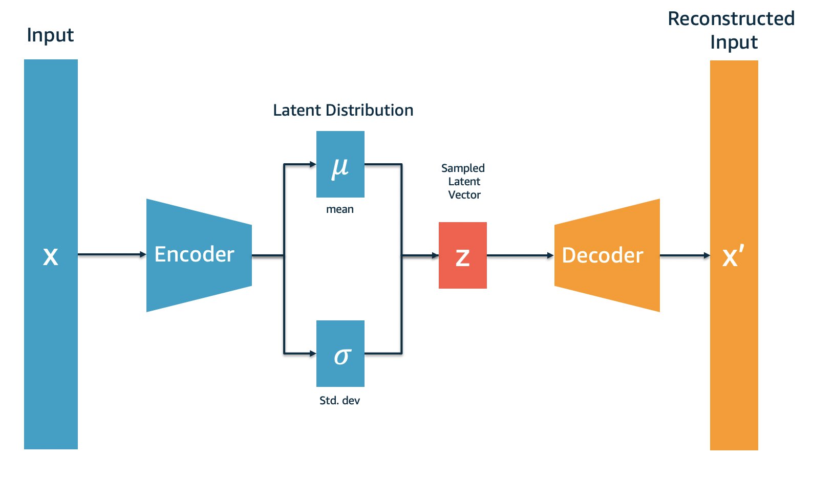
Abstract diagram of a VAE, pilfered from this AWS blog

Our goal is to implement the model code for the VAE as well as the training loop with both the reconstruction and variational loss terms. Then, we can sample new digits that look like those in the MNIST dataset! Additionally, we will provide an extra input to the model – the class index – so we can control which number we want to generate.

Let’s begin by defining our configuration. For this educational example, we will just define some constants in a cell:

batch_size = 16
latent_dim = 32
kl_weight = 0.5
num_classes = 10
seed = 0xffff

Along with some imports and PRNG initialisation:

import jax # install correct wheel for accelerator you want to use
import flax
import optax
import orbax

import flax.linen as nn
import jax.numpy as jnp
import numpy as np
from jax.typing import ArrayLike

from typing import Tuple, Callable
from math import sqrt

import torchvision.transforms as T
from torchvision.datasets import MNIST
from torch.utils.data import DataLoader

key = jax.random.PRNGKey(seed)

Let’s grab our MNIST dataset while we are here:

train_dataset = MNIST('data', train = True, transform=T.ToTensor(), download=True)
train_loader = DataLoader(train_dataset, batch_size=batch_size, shuffle=True, drop_last=True)

JAX, Flax, and Optax do not have data loading utilities, so I just use the perfectly serviceable PyTorch implementation of the MNIST dataset here.

Now to our first real Flax model. We begin by defining a submodule FeedForward that implements a stack of linear layers with intermediate non-linearities:

class FeedForward(nn.Module):
  dimensions: Tuple[int] = (256, 128, 64)
  activation_fn: Callable = nn.relu
  drop_last_activation: bool = False

  @nn.compact
  def __call__(self, x: ArrayLike) -> ArrayLike:
    for i, d in enumerate(self.dimensions):
      x = nn.Dense(d)(x)  
      if i != len(self.dimensions) - 1 or not self.drop_last_activation:
        x = self.activation_fn(x)
    return x

key, model_key = jax.random.split(key)
model = FeedForward(dimensions = (4, 2, 1), drop_last_activation = True)
print(model)

params = model.init(model_key, jnp.zeros((1, 8)))
print(params)

key, x_key = jax.random.split(key)
x = jax.random.normal(x_key, (1, 8))
y = model.apply(params, x)

y
===
Out: 


FeedForward(
    # attributes
    dimensions = (4, 2, 1)
    activation_fn = relu
    drop_last_activation = True
)
FrozenDict({
    params: {
        Dense_0: {
            kernel: Array([[ 0.0840368 , -0.18825287,  0.49946404, -0.4610112 ],
                   [ 0.4370267 ,  0.21035315, -0.19604324,  0.39427406],
                   [ 0.00632685, -0.02732705,  0.16799504, -0.44181877],
                   [ 0.26044282,  0.42476758, -0.14758752, -0.29886967],
                   [-0.57811564, -0.18126923, -0.19411889, -0.10860331],
                   [-0.20605426, -0.16065307, -0.3016759 ,  0.44704655],
                   [ 0.35531637, -0.14256613,  0.13841921,  0.11269159],
                   [-0.430825  , -0.0171169 , -0.52949774,  0.4862139 ]],      dtype=float32),
            bias: Array([0., 0., 0., 0.], dtype=float32),
        },
        Dense_1: {
            kernel: Array([[ 0.03389561, -0.00805947],
                   [ 0.47362345,  0.37944487],
                   [ 0.41766328, -0.15580587],
                   [ 0.5538078 ,  0.18003668]], dtype=float32),
            bias: Array([0., 0.], dtype=float32),
        },
        Dense_2: {
            kernel: Array([[ 1.175035 ],
                   [-1.1607001]], dtype=float32),
            bias: Array([0.], dtype=float32),
        },
    },
})

Array([[0.5336972]], dtype=float32)

We use the nn.compact decorator here as the logic is relatively simple. We iterate over the tuple self.dimensions and pass our current activations through a nn.Dense module, followed by applying self.activation_fn. This activation can optionally be dropped for the final linear layer in FeedForward. This is needed as nn.relu only outputs non-negative values, whereas sometimes we need non-negative outputs!

Using FeedForward, we can define our full VAE model:

class VAE(nn.Module):
  encoder_dimensions: Tuple[int] = (256, 128, 64)
  decoder_dimensions: Tuple[int] = (128, 256, 784)
  latent_dim: int = 4
  activation_fn: Callable = nn.relu

  def setup(self):
    self.encoder = FeedForward(self.encoder_dimensions, self.activation_fn)
    self.pre_latent_proj = nn.Dense(self.latent_dim * 2)
    self.post_latent_proj = nn.Dense(self.encoder_dimensions[-1])
    self.class_proj = nn.Dense(self.encoder_dimensions[-1])
    self.decoder = FeedForward(self.decoder_dimensions, self.activation_fn, drop_last_activation=False)

  def reparam(self, mean: ArrayLike, logvar: ArrayLike, key: jax.random.PRNGKey) -> ArrayLike:
    std = jnp.exp(logvar * 0.5)
    eps = jax.random.normal(key, mean.shape)
    return eps * std + mean

  def encode(self, x: ArrayLike):
    x = self.encoder(x)
    mean, logvar = jnp.split(self.pre_latent_proj(x), 2, axis=-1)
    return mean, logvar

  def decode(self, x: ArrayLike, c: ArrayLike):
    x = self.post_latent_proj(x)
    x = x + self.class_proj(c)
    x = self.decoder(x)
    return x

  def __call__(
      self, x: ArrayLike, c: ArrayLike, key: jax.random.PRNGKey) -> Tuple[ArrayLike, ArrayLike, ArrayLike]:
    mean, logvar = self.encode(x)
    z = self.reparam(mean, logvar, key)
    y = self.decode(z, c)
    return y, mean, logvar

key = jax.random.PRNGKey(0x1234)
key, model_key = jax.random.split(key)
model = VAE(latent_dim=4)
print(model)

key, call_key = jax.random.split(key)
params = model.init(model_key, jnp.zeros((batch_size, 784)), jnp.zeros((batch_size, num_classes)), call_key)

recon, mean, logvar = model.apply(params, jnp.zeros((batch_size, 784)), jnp.zeros((batch_size, num_classes)), call_key)
recon.shape, mean.shape, logvar.shape
===
Out:
ClassVAE(
    # attributes
    encoder_dimensions = (256, 128, 64)
    decoder_dimensions = (128, 256, 784)
    latent_dim = 4
    activation_fn = relu
)
((16, 784), (16, 4), (16, 4))

There is a lot to the above cell. Knowing the specifics of how this model works isn’t too important to understanding the training loop later, as we can treat the model as a bit of a black box. Simply substitute your own model of choice. Saying that, I’ll unpack each function briefly:

• setup: Creates the submodules of the network, namely two FeedForward stacks and two nn.Linear layers that project to and from the latent space. Additionally, it initialises a third nn.Linear layer that projects our class conditioning vector to the same dimensionality as the last encoder layer.
• reparam: Sampling a latent directly from a random Gaussian is not differentiable, hence we employ the reparameterisation trick. This involves sampling a random vector, scaling by the standard deviation, then adding to the mean. As it involves random array generation, we take as input a key in addition to the mean and log-variance.
• encode: Applies the encoder and projection to the latent space to the input. Note, the output of the projection is actually double the size of the latent space, as we split it in twine to obtain our mean and log-variance.
• decode: Applies a projection from the latent space to x, followed by adding the output of class_proj on the conditioning vector. This is how we inject the class information into the model. Finally, it passes the result through the decoder stack.
• __call__: This is simply the full model forward pass: encode then reparam then decode. This is used during training.

The above example also demonstrates that we can add other functions to our Flax modules aside from setup and __call__. This is useful for more complex behaviour, or if we want to only execute parts of the model (more on this later).

We now have our model, optimiser, and dataset. The next step is to write the function that implements our training step and then jit-compile it:

def create_train_step(key, model, optimiser):
  params = model.init(key, jnp.zeros((batch_size, 784)), jnp.zeros((batch_size, num_classes)), jax.random.PRNGKey(0)) # dummy key just as example input
  opt_state = optimiser.init(params)
  
  def loss_fn(params, x, c, key):
    reduce_dims = list(range(1, len(x.shape)))
    c = jax.nn.one_hot(c, num_classes) # one hot encode the class index
    recon, mean, logvar = model.apply(params, x, c, key)
    mse_loss = optax.l2_loss(recon, x).sum(axis=reduce_dims).mean()
    kl_loss = jnp.mean(-0.5 * jnp.sum(1 + logvar - mean ** 2 - jnp.exp(logvar), axis=reduce_dims)) # KL loss term to keep encoder output close to standard normal distribution.

    loss = mse_loss + kl_weight * kl_loss
    return loss, (mse_loss, kl_loss)

  @jax.jit
  def train_step(params, opt_state, x, c, key):
    losses, grads = jax.value_and_grad(loss_fn, has_aux=True)(params, x, c, key)
    loss, (mse_loss, kl_loss) = losses
    
    updates, opt_state = optimiser.update(grads, opt_state, params)
    params = optax.apply_updates(params, updates)

    return params, opt_state, loss, mse_loss, kl_loss

  return train_step, params, opt_state

Here, I don’t define the training step directly, but rather define a function that returns the training step function given a target model and optimiser, along with returning the freshly initialised parameters and optimiser state.

Let us unpack it all:

1. First, it initialises our model using an example input. In this case, this is a 784-dim array which contains the (flattened) MNIST digit and a random, random key.
2. Also initialises the optimiser state using the parameters we just initialised.
3. Now, it defines the loss function. This is simply a model.apply call which returns the model’s reconstruction of the input, along with the predicted mean and log-variance. We then compute the mean-squared error loss and the KL-divergence, before finally computing a weighted sum to get our final loss. The KL loss term is what keeps the encoder outputs close to a standard normal distribution.
4. Next, the actual train step definition. This begins by transforming loss_fn using our old friend jax.value_and_grad which will return the loss and also the gradients. We must set has_aux=True as we return all individual loss terms for logging purposes. We provide the gradients, optimiser state, and parameters to optimiser.update which returns the transformed gradients and the new optimiser state. The transformed gradients are then applied to the parameters. Finally, we return the new parameters, optimiser state, and loss terms – followed by wrapping the whole thing in jax.jit. Phew..

A function that generates the training step is just a pattern I quite like, and there is nothing stopping you from just writing the training step directly.

Let’s call create_train_step:

key, model_key = jax.random.split(key)

model = VAE(latent_dim=latent_dim)
optimiser = optax.adamw(learning_rate=1e-4)

train_step, params, opt_state = create_train_step(model_key, model, optimiser)

When we call the above, we get a train_step ready to be compiled and accept our parameters, optimiser state, and data at blistering fast speeds. As always with jit-compiled functions, the first call with a given set of input shapes will be slow, but fast on subsequent calls as we skip the compiling and optimisation process.

We are now in a position to write our training loop and train the model!

freq = 100
for epoch in range(10):
  total_loss, total_mse, total_kl = 0.0, 0.0, 0.0
  for i, (batch, c) in enumerate(train_loader):
    key, subkey = jax.random.split(key)

    batch = batch.numpy().reshape(batch_size, 784)
    c = c.numpy()
    params, opt_state, loss, mse_loss, kl_loss = train_step(params, opt_state, batch, c, subkey)

    total_loss += loss
    total_mse += mse_loss
    total_kl += kl_loss

    if i > 0 and not i % freq:
      print(f"epoch {epoch} | step {i} | loss: {total_loss / freq} ~ mse: {total_mse / freq}. kl: {total_kl / freq}")
      total_loss = 0.
      total_mse, total_kl = 0.0, 0.0
===
Out:
epoch 0 | step 100 | loss: 49.439998626708984 ~ mse: 49.060447692871094. kl: 0.7591156363487244
epoch 0 | step 200 | loss: 37.1823616027832 ~ mse: 36.82903289794922. kl: 0.7066375613212585
epoch 0 | step 300 | loss: 33.82365036010742 ~ mse: 33.49456024169922. kl: 0.6581906080245972
epoch 0 | step 400 | loss: 31.904821395874023 ~ mse: 31.570871353149414. kl: 0.6679074764251709
epoch 0 | step 500 | loss: 31.095705032348633 ~ mse: 30.763246536254883. kl: 0.6649144887924194
epoch 0 | step 600 | loss: 29.771989822387695 ~ mse: 29.42426872253418. kl: 0.6954278349876404

...

epoch 9 | step 3100 | loss: 14.035745620727539 ~ mse: 10.833460807800293. kl: 6.404574871063232
epoch 9 | step 3200 | loss: 14.31241226196289 ~ mse: 11.043667793273926. kl: 6.53748893737793
epoch 9 | step 3300 | loss: 14.26440143585205 ~ mse: 11.01070785522461. kl: 6.5073771476745605
epoch 9 | step 3400 | loss: 13.96005630493164 ~ mse: 10.816412925720215. kl: 6.28728723526001
epoch 9 | step 3500 | loss: 14.166285514831543 ~ mse: 10.919700622558594. kl: 6.493169784545898
epoch 9 | step 3600 | loss: 13.819541931152344 ~ mse: 10.632755279541016. kl: 6.373570919036865
epoch 9 | step 3700 | loss: 14.452215194702148 ~ mse: 11.186063766479492. kl: 6.532294750213623

Now that we have our train_step function, the training loop itself is just repeatedly fetching data, calling our uber-fast train_step function, and logging results so we can track training. We can see that the loss is decreasing, which means our model is training!

Note that the KL-loss term increases during training. This is okay so long as it doesn’t get too high, in which case sampling from the model becomes impossible. Tuning the hyperparameter kl_weight is quite important. Too low and we get perfect reconstructions but no sampling capabilities – too high and the outputs will become blurry.

Let’s sample from the model so we can see that it does indeed produce some reasonable samples:

def build_sample_fn(model, params):
  @jax.jit
  def sample_fn(z: jnp.array, c: jnp.array) -> jnp.array:
    return model.apply(params, z, c, method=model.decode)
  return sample_fn

sample_fn = build_sample_fn(model, params)

num_samples = 100
h, w = 10

key, z_key = jax.random.split(key)
z = jax.random.normal(z_key, (num_samples, latent_dim))
c = np.repeat(np.arange(h)[:, np.newaxis], w, axis=-1).flatten()
c = jax.nn.one_hot(c, num_classes)
sample = sample_fn(z, c)
z.shape, c.shape, sample.shape
===
Out: ((100, 32), (100, 10), (100, 784))

The above cell generates 100 samples – 10 examples from each of the 10 classes. We jit-compile our sample function in case we want to sample again later. We only call the model.decode method, rather than the full model, as we only need to decode our randomly sampled latents. This is achieved by specifying method=model.decode in the model.apply call.

Let’s visualise the results using matplotlib:

import matplotlib.pyplot as plt
import math
from numpy import einsum

sample = einsum('ikjl', np.asarray(sample).reshape(h, w, 28, 28)).reshape(28*h, 28*w)

plt.imshow(sample, cmap='gray')
plt.show()

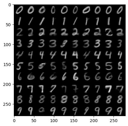
It seems our model did indeed train and can be sampled from! Additionally, the model is capable of using the class conditioning signal so that we can control which digits are generated. Therefore, we have succeeded in building a full training loop using Flax and Optax!

Extra Flax and Optax Tidbits

I’d like to finish this blog post by highlighting some interesting and useful features that may prove useful in your own applications. I won’t delve into great detail with any of them, but simply summarise and point you in the right direction.

You may have noticed already that when we add parameters, optimiser states, and a bunch of other metrics to the return call of train_step it gets a bit unwieldy to handle all the state. It could get worse if we later need a more complex state. One solution would be to return a namedtuple so we can at least package the state together somewhat. However, Flax provides its own solution, flax.training.train_state.TrainState, which has some extra functions that make updating the combined state (model and optimiser state) easier.

It is easiest to show by simply taking our earlier train_step and refactoring it with TrainState:

from flax.training.train_state import TrainState
def create_train_step(key, model, optimiser):
  params = model.init(key, jnp.zeros((batch_size, 784)), jnp.zeros((batch_size, num_classes)), jax.random.PRNGKey(0))
  state = TrainState.create(apply_fn=model.apply, params=params, tx=optimiser)
  
  def loss_fn(state, x, c, key):
    reduce_dims = list(range(1, len(x.shape)))
    c = jax.nn.one_hot(c, num_classes)
    recon, mean, logvar = state.apply_fn(state.params, x, c, key)
    mse_loss = optax.l2_loss(recon, x).sum(axis=reduce_dims).mean()
    kl_loss = jnp.mean(-0.5 * jnp.sum(1 + logvar - mean ** 2 - jnp.exp(logvar), axis=reduce_dims))

    loss = mse_loss + kl_weight * kl_loss
    return loss, (mse_loss, kl_loss)

  @jax.jit
  def train_step(state, x, c, key):
    losses, grads = jax.value_and_grad(loss_fn, has_aux=True)(state, x, c, key)
    loss, (mse_loss, kl_loss) = losses

    state = state.apply_gradients(grads=grads)

    return state, loss, mse_loss, kl_loss

  return train_step, state

We begin create_train_step by initialising our parameters as before. However, the next step is now to create the state using TrainState.create and passing our model forward call, the initialised parameters, and the optimiser we want to use. Internally, TrainState.create will initialise and store the optimiser state for us.

In loss_fn, rather than call model.apply we can use state.apply_fn instead. Either method is equivalent, just that sometimes we may not have model in scope and so can’t access model.apply.

The largest change is in train_step itself. Rather than call optimiser.update followed by optax.apply_updates, we simply call state.apply_gradients which internally updates the optimiser state and the parameters. It then returns the new state, which we return and pass to the next call of train_step – as we would with params and opt_state.

It is possible to add extra attributes to TrainState by subclassing it, for example adding attributes to store the latest loss.

In conclusion, TrainState makes it easier to pass around state in the training loop, as well as abstracting away optimiser and parameter updates.

Another useful feature of Flax is the ability to bind parameters to a model, yielding an interactive instance that can be called directly, as if it were a PyTorch model with internal state. However, this state is static and can only change if we bind it again, which makes it unusable for training. However, it can be handy for interactive debugging or inference.

The API is pretty simple:

key, model_key = jax.random.split(key)
model = nn.Dense(2)
params = model.init(model_key, jnp.zeros(8))

bound_model = model.bind(params)
bound_model(jnp.ones(8))
===
Out: Array([ 0.45935923, -0.691003  ], dtype=float32)

We can get back the unbound model and its parameters by calling model.unbind:

bound_model.unbind()
===
Out: (Dense(
     # attributes
     features = 2
     use_bias = True
     dtype = None
     param_dtype = float32
     precision = None
     kernel_init = init
     bias_init = zeros
     dot_general = dot_general
 ),
 FrozenDict({
     params: {
         kernel: Array([[-0.11450272, -0.2808447 ],
                [-0.45104247, -0.3774913 ],
                [ 0.07462895,  0.3622056 ],
                [ 0.59189916, -0.34050766],
                [-0.10401642, -0.36226135],
                [ 0.157985  ,  0.00198693],
                [-0.00792678, -0.1142673 ],
                [ 0.31233454,  0.4201768 ]], dtype=float32),
         bias: Array([0., 0.], dtype=float32),
     },
 }))

I said I wouldn’t enumerate layers in Flax as I don’t see much value in doing so, but I will highlight two particularly interesting ones. First is nn.Dropout which is numerically the same as its PyTorch counterpart, but like anything random in JAX, requires a PRNG key as input.

The dropout layer takes its random key by internally calling self.make_rng('dropout'), which pulls and splits from a PRNG stream named 'dropout'. This means when we call model.apply we will need to define the starting key for this PRNG stream. This can be done by passing a dictionary mapping stream names to PRNG keys, to the rngs argument in model.apply:

key, x_key = jax.random.split(key)
key, drop_key = jax.random.split(key)
x = jax.random.normal(x_key, (3,3))

model = nn.Dropout(0.5, deterministic=False)
y = model.apply({}, x, rngs={'dropout': drop_key}) # there is no state, just pass empty dictionary :)
x, y
===
Out: (Array([[ 1.7353934, -1.741734 , -1.3312583],
        [-1.615281 , -0.6381292,  1.3057163],
        [ 1.2640097, -1.986926 ,  1.7818599]], dtype=float32),
 Array([[ 3.4707868,  0.       , -2.6625166],
        [ 0.       ,  0.       ,  2.6114326],
        [ 0.       , -3.973852 ,  0.       ]], dtype=float32))

model.init also accepts a dictionary of PRNG keys. If you pass in a single key like we have done so far, it starts a stream named 'params'. This is equivalent to passing {'params': rng} instead.

The streams are accessible to submodules, so nn.Dropout can call self.make_rng('dropout') regardless of where it is in the model. We can define our own PRNG streams by specifying them in the model.apply call. In our VAE example, we could forgo passing in the key manually, and instead get keys for random sampling using self.make_rng('noise') or similar, then passing a starting key in rngs in model.apply. For models with lots of randomness, it may be worth doing this.

The second useful built-in module is nn.Sequential which is again like its PyTorch counterpart. This simply chains together many modules such that the outputs of one module will flow into the inputs of the next. Useful if we want to define large stacks of layers quickly.

Now onto some Optax tidbits! First, Optax comes with a bunch of learning rate schedulers. Instead of passing a float value to learning_rate when creating the optimiser, we can pass a scheduler. When applying updates, Optax will automatically select the correct learning rate. Let’s define a simple, linear schedule:

start_lr, end_lr = 1e-3, 1e-5
steps = 10_000
lr_scheduler = optax.linear_schedule(
  init_value=start_lr,
  end_value=end_lr,
  transition_steps=steps,
)
optimiser = optax.adam(learning_rate=lr_scheduler)

You can join together schedulers using optax.join_schedules in order to get more complex behaviour like learning rate warmup followed by decay:

warmup_start_lr, warmup_steps = 1e-6, 1000
start_lr, end_lr, steps = 1e-2, 1e-5, 10_000
lr_scheduler = optax.join_schedules(
    [
        optax.linear_schedule(
            warmup_start_lr,
            start_lr,
            warmup_steps,
        ),
        optax.linear_schedule(
            start_lr,
            end_lr,
            steps - warmup_steps,
        ),
    ],
    [warmup_steps],
)

optimiser = optax.adam(lr_scheduler)

The last argument to optax.join_schedules should be a sequence of integers defining the step boundaries between different schedules. In this case, we switch from warmup to decay after warmup_steps steps.

Optax keeps track of the number of optimiser steps in its opt_state, so we don’t need to track this ourselves. It will use this count to automatically pick the correct learning rate.

Similar to joining schedulers, Optax supports chaining optimisers together. More specifically, the chaining of gradient transformations:

optimiser = optax.chain(
    optax.clip_by_global_norm(1.0),
    optax.adam(1e-2),
)

When calling optimiser.update, the gradients will first be clipped before then doing the regular Adam update. Chaining together transformations like this is quite an elegant API and allows for complex behaviour. To illustrate, adding exponential moving averages (EMA) of our updates in something like PyTorch is non-trivial, whereas in Optax it is as simple as adding optax.ema to our optax.chain call:

optimiser = optax.chain(
    optax.clip_by_global_norm(1.0),
    optax.adam(1e-2),
    optax.ema(decay=0.999)
)

In this case, optax.ema is a transformation on the final updates, rather than on the unprocessed gradients.

Gradient accumulation is implemented in Optax as a optimiser wrapper, rather than as a gradient transformation:

grad_accum = 4
optimiser = optax.MultiSteps(optax.adam(1e-2), grad_accum)

The returned optimiser collects updates over the optimiser.update calls until grad_accum steps have occurred. In the intermediate steps, the returned updates will be a PyTree of zeros in the same shape as params, resulting in no update. Every grad_accum steps, the accumulated updates will be returned.

grad_accum can also be a function, which gives us a way to vary the batch size during training via adjusting the number of steps between parameter updates.

How about if we only want to train certain parameters? For example, when finetuning a pretrained model. Nowadays, this is a pretty common thing to do, taking pretrained large language models and adapting them for specific downstream tasks.

Let’s grab a pretrained BERT model from the Huggingface hub:

from transformers import FlaxBertForSequenceClassification
model = FlaxBertForSequenceClassification.from_pretrained('bert-base-uncased')
model.params.keys()
===
Out: dict_keys(['bert', 'classifier'])

Huggingface provides Flax versions of most of their models. The API to use them is a bit different, calling model(**inputs, params=params) rather than model.apply. Providing no parameters will use the pretrained weights stored in model.params which is useful for inference-only tasks, but for training we need to pass the current parameters to the call.

We can see there are two top-level keys in the parameter PyTree: bert and classifier. Suppose we only want to finetune the classifier head and leave the BERT backbone alone, we can achieve this using optax.multi_transform:

optimiser = optax.multi_transform({'train': optax.adam(1e-3), 'freeze': optax.set_to_zero()}, {'bert': 'freeze', 'classifier': 'train'})
opt_state = optimiser.init(model.params)

grads = jax.tree_map(jnp.ones_like, model.params)
updates, opt_state = optimiser.update(grads, opt_state, model.params)

optax.multi_transform takes two inputs, the first is mapping from labels to gradient transformations. The second is a PyTree with the same structure or prefix as the updates (in the case above we use the prefix approach) mapping to labels. The transformation matching the label of a given update will be applied. This allows the partitioning of parameters and applying different updates to different parts.

The second argument can also be a function that, given the updates PyTree, returns such a PyTree mapping updates (or their prefix) to labels.

This can be used for other cases like having different optimisers for different layers (such as disabling weight decay for certain layers), but in our case we simply use optax.adam for our trainable parameters, and zero out gradients for other regions using the stateless transform optax.set_to_zero.

In jit-compiled function, the gradients that have optax.set_to_zero applied to them won’t be computed due to the optimisation process seeing that they will always be zero. Hence, we get the expected memory savings from only finetuning a subset of layers!

Let’s print the updates so that we can see that we do indeed have no updates in the BERT backbone, and have updates in the classifier head:

updates['classifier'], updates['bert']['embeddings']['token_type_embeddings']
===
Out:
{'bias': Array([-0.00100002, -0.00100002], dtype=float32),
 'kernel': Array([[-0.00100002, -0.00100002],
        [-0.00100002, -0.00100002],
        [-0.00100002, -0.00100002],
        ...,
        [-0.00100002, -0.00100002],
        [-0.00100002, -0.00100002],
        [-0.00100002, -0.00100002]], dtype=float32)}
{'embedding': Array([[0., 0., 0., ..., 0., 0., 0.],
        [0., 0., 0., ..., 0., 0., 0.]], dtype=float32)}

We can verify that all updates are zero using jax.tree_util.tree_reduce:

jax.tree_util.tree_reduce(lambda c, p: c and (jnp.count_nonzero(p) == 0), updates['bert'], True)
===
Out: Array(True, dtype=bool)

Both Flax and Optax are quite feature-rich despite the relative infancy of the JAX ecosystem. I’d recommend just opening the Flax or Optax API reference and searching for layers, optimisers, loss functions, and features you are used to having in other frameworks.

The last thing I want to talk about involves an entirely different library built on JAX. Orbax provides PyTree checkpointing utilities for saving and restoring arbitrary PyTrees. I won’t go into great detail but will show basic usage here. There is nothing worse than spending hours training only to realise you forgot to add checkpointing code!

Here is basic usage saving the BERT classifier parameters:

import orbax
import orbax.checkpoint
from flax.training import orbax_utils

orbax_checkpointer = orbax.checkpoint.PyTreeCheckpointer()
save_args = orbax_utils.save_args_from_target(model.params['classifier'])
orbax_checkpointer.save('classifier.ckpt', model.params['classifier'], save_args=save_args)
!ls
===
Out: classifier.ckpt

Which we can restore by executing:

orbax_checkpointer.restore('classifier.ckpt')
===
Out: {'bias': array([0., 0.], dtype=float32),
 'kernel': array([[-0.06871808, -0.06338844],
        [-0.03397266,  0.00899913],
        [-0.00669084, -0.06431466],
        ...,
        [-0.02699363, -0.03812294],
        [-0.00148801,  0.01149782],
        [-0.01051403, -0.00801195]], dtype=float32)}

Which returns the raw PyTree. If you are using a custom dataclass with objects that can’t be serialised (such as a Flax train state where apply_fn and tx can’t be serialised) you can pass a dummy PyTree of the same structure as the saved one using the item argument in the restore call, to let Orbax know the structure you want.

You can read more about restoring custom dataclasses here in the Orbax documentation

Manually saving checkpoints like this is a bit old-fashioned. Orbax has a bunch of automatic versioning and scheduling features built in, such as automatic deleting of old checkpoints, tracking the best metric, and more. To use these features, wrap the orbax_checkpointer in orbax.checkpoint.CheckpointManager:

options = orbax.checkpoint.CheckpointManagerOptions(max_to_keep=4, create=True)
checkpoint_manager = orbax.checkpoint.CheckpointManager(
    'managed-checkpoint', orbax_checkpointer, options)

for step in range(10):
    checkpoint_manager.save(step, model.params['classifier'], save_kwargs={'save_args': save_args})

!ls -l managed-checkpoint/*
===
Out:
managed-checkpoint/6:
total 4
drwxr-xr-x 2 root root 4096 Jun  3 09:07 default

managed-checkpoint/7:
total 4
drwxr-xr-x 2 root root 4096 Jun  3 09:07 default

managed-checkpoint/8:
total 4
drwxr-xr-x 2 root root 4096 Jun  3 09:07 default

managed-checkpoint/9:
total 4
drwxr-xr-x 2 root root 4096 Jun  3 09:07 default

As we set max_to_keep=4, only the last four checkpoints have been kept.

We can view which steps have checkpoints:

checkpoint_manager.all_steps()
===
Out: [6, 7, 8, 9]

As well as view if there is a checkpoint for a specific step:

checkpoint_manager.should_save(6)
===
Out: False

And what the latest saved step was:

checkpoint_manager.latest_step()
===
Out: 9

We can restore using the checkpoint manager. Rather than provide a path to the restore function, we provide the step we want to restore:

step = checkpoint_manager.latest_step()
checkpoint_manager.restore(step)
===
Out: {'bias': array([0., 0.], dtype=float32),
 'kernel': array([[-0.06871808, -0.06338844],
        [-0.03397266,  0.00899913],
        [-0.00669084, -0.06431466],
        ...,
        [-0.02699363, -0.03812294],
        [-0.00148801,  0.01149782],
        [-0.01051403, -0.00801195]], dtype=float32)}

For especially large checkpoints, Orbax supports asynchronous checkpointing which moves checkpointing to a background thread. You can do this by wrapping orbax.checkpoint.AsyncCheckpointer around the orbax.checkpoint.PyTreeCheckpointer we created earlier.

You may see reference online to Flax checkpointing utilities. However, these utilities are being deprecated and it is recommended to start using Orbax instead.

The documentation for Orbax is a bit spartan, but it has a fair few options to choose. It is worth just reading the CheckpointManagerOptions class here and seeing the available features.

Conclusion

In this blog post, I’ve introduced two libraries built on top of JAX: Flax and Optax. This has been more of a practical guide into how you can implement training loops easily in JAX using these libraries, rather than a ideological discussion like my previous blog post on JAX.

To summarise this post:

• Flax provides a neural network API that allows the developer to build neural network modules in a class-based way. Unlike other frameworks, these modules do not contain state within them, essentially hollow shells that loosely associate functions with parameters and inputs, and provide easy methods to initialise the parameters.
• Optax provides a large suite of optimisers for updating our parameters. These, like Flax modules, do not contain state and must have state passed manually to it. All optimisers are simply gradient transformations: a pair of pure functions init and update. Optax also provides other gradient transformations and wrappers to allow for more complex behaviour, such as gradient clipping and parameter freezing.
• Both libraries simply operate on and return PyTrees and can easily interoperate with base JAX — crucially with jax.jit. This also makes them interoperable with other libraries based on JAX. For example, by choosing Flax, we aren’t locked into using Optax, and vice versa.

There is a lot more to these two libraries than described here, but I hope this is a good starting point and can enable you to create your own training loops in JAX. A good exercise now would be to use the training loop and model code in this blog post and adapting it for your own tasks, such as another generative model.

If you liked this post please consider following me on Twitter or use this site’s RSS feed for notifications on future ramblings about machine learning and other topics. Alternatively you can navigate to the root of this website and repeatedly refresh until something happens. Thank you for reading this far and I hope you found it useful!

Acknowledgements and Extra Resources

Some good extra resources:

• My previous blog post on JAX
• Aleksa Gordic’s JAX and Flax tutorial series
• Flax documentation
• Optax documentation
• Orbax source code

Some alternatives to Flax:

• Equinox by Patrick Kidger
• Haiku from Deepmind

I am not aware of relatively mature alternatives to Optax. If you know of some, please let me know!

Found something wrong with this blog post? Let me know via email or Twitter!